This article assumes little to no prior knowledge about Azure AI Services, however does assume basic knowledge about Azure itself, as well as AI in general.

Microsoft’s Azure AI Platform offers various solutions and tools for the purpose of rapidly developing Artificial Intelligence (AI) projects, i.e., any projects that involve some form of AI. It offers tooling for common problem spaces, such as vision, speech and translation. [1]

One key feature of Azure AI is that it can be used both through SDK’s in various languages — such as Python, Rust or C# — or through regular HTTP calls to a REST endpoint. Through one of these methods, AI can easily be incorporated into both existing and new projects.

In this blog post we will be looking up at setting up a simple Azure AI-powered application that downloads, caches and then analyzes an image, using Python. In particular, we will look at Azure AI Vision, which provides access to image processing algorithms. This can be useful for purposes such as automatically assigning tags to images. [2]

For simplicity, let us make the following assumptions:

• All input, other than ‘quit’, is a valid URL. There is no explicit URL validation.
• Errors can occur in a very limited number of situations, meaning that we only explicitly handle exceptions when absolutely needed.

CREATING AZURE RESOURCES

There are various ways of setting up an Azure AI Vision service. It is possible to create a multi-service AI resource, which offers access to multiple AI services at a given time, or a single-service AI resource, which offers access to just one, such as vision or speech. Which option to pick can differ based on factors such as whether the billing should be separate for each AI service. For now, let us proceed by creating a multi-service resource.

To create such a resource, open the Azure Portal and create a new resource. In the marketplace, search for azure ai services and select the corresponding resource. Figure 1 shows the resource you should pick.

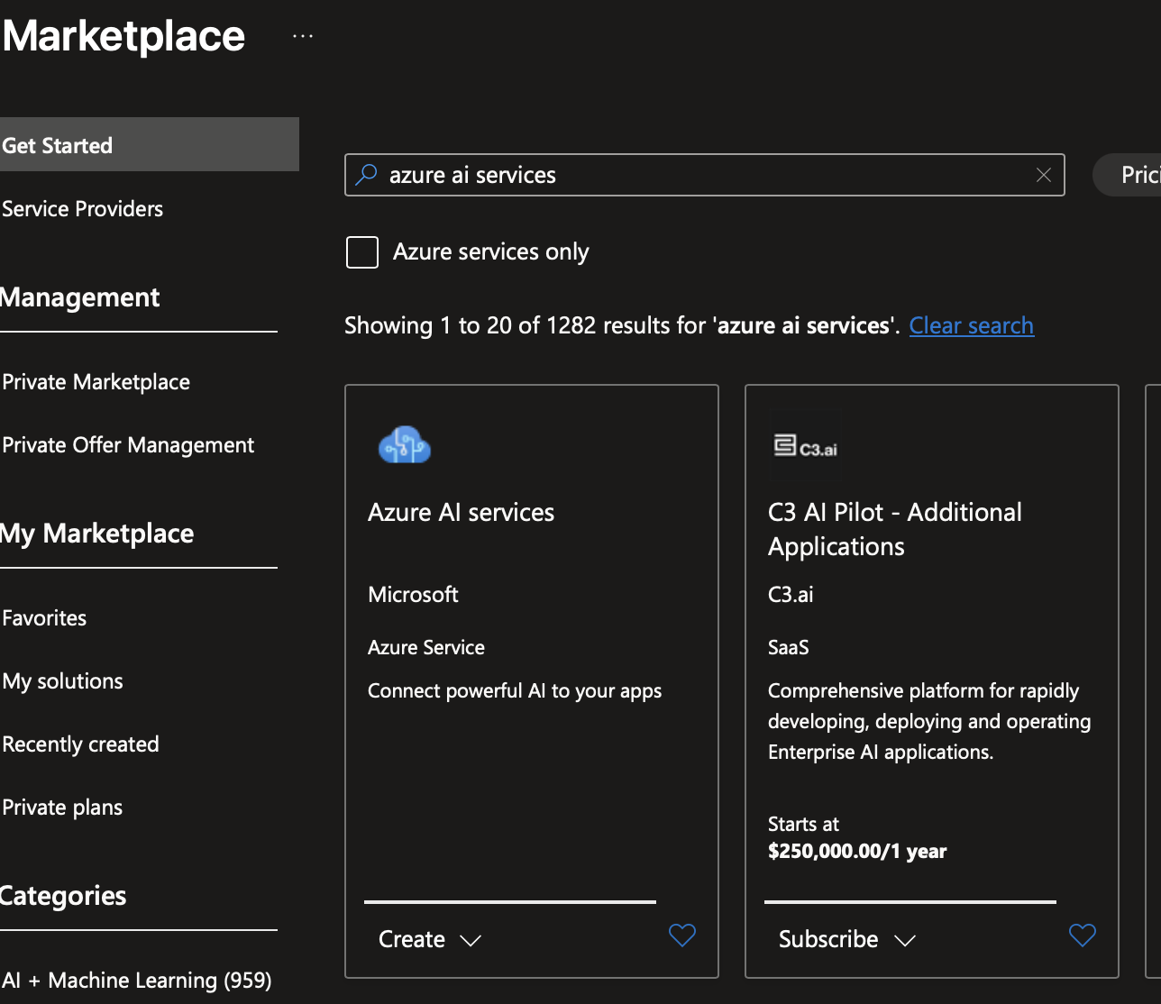
Click on the create button. Let us ignore the network configuration for now and simply specify a resource group, pricing tier and a name. For example:

• Subscription: armonden-main
• Resource group: armonden-platform-dev-rg
• Name: armonden-platform-dev-ai
• Pricing tier: Standard S0

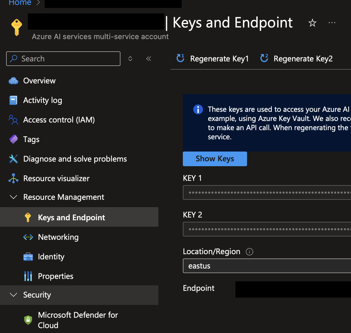
On the resource overview page, go to Keys and Endpoint. This page lists two keys and an endpoint. Both the key and endpoint are required to set up the client. It does not matter which key you select, since both can be used. One typical use case would be to use one key for a development environment and the other for production.¹ Figure 2 shows an example of the keys and endpoint page of a multi-service account.

SETTING UP THE AZURE AI VISION CLIENT

To create an Azure AI Vision client using Python, first create a new folder, with a .env file. For now it suffices to use this file to store the configuration. The contents of this file should look similar to the following file:

AI_SERVICE_ENDPOINT=https://ai-services-resource.cognitiveservices.azure.com/
AI_SERVICE_KEY=ai_services_key

The exact configuration is determined by the values retrieved from the keys and endpoint page. Now, set up a Python virtual environment by running the following commands in a terminal:

$ python3 -m venv .venv
$ ./.venv/bin/activate

Now that a virtual environment has been set up and activate, it is time to download the dependencies. For this simple example, install the following packages using Pip:

• dotenv (at version 0.9.9 or higher)
• azure-ai-vision-imageanalysis (at version 1.0.0 or higher)
• requests (at version 2.32.3 or higher)

Once these packages have been installed, let us move on to the implementation of the client itself. The gameplay loop of the client is very simple. Considering a happy path, it behaves in the following manner:

1. Read some input \(x\) from the user.
2. If \(x=\)'q', then stop the program.
3. Calculate some hash \(x_\text{hashed}\) based on the input.
4. If \(x_\text{hashed}\notin\text{cache}\), then download the image and store it in the cache.
5. Perform image analysis on file \(x_\text{hashed}\).
6. Print the results to console.
7. Return to 1.

IMPLEMENTING THE CLIENT

Now, it is time to move on to the code. Create a new python file, e.g., client.py. Then add the following imports, such that the top of the file looks as follows:

#!/usr/bin/env python3

from os import getenv, path, makedirs

from dotenv import load_dotenv
from requests import get

from azure.ai.vision.imageanalysis import ImageAnalysisClient
from azure.ai.vision.imageanalysis.models import VisualFeatures
from azure.core.credentials import AzureKeyCredential

Note that I have included a shebang to avoid the need to type python3 client.py, however this is merely personal preference and is not required.² If you include it, ensure that it points to the correct binary: on Windows, for example, python3 may not exist and instead be referred to as simply python. In this case, update the shebang accordingly.³

Now let us implement a basic loop that reads user input and calls a function that, given a vision client and a URL, runs an image analysis. For good measure, we also set up stub for the vision client loading function. The code, as you would expect, is quite trivial:

def run_analysis_on_url(client: ImageAnalysisClient, url: str):
    pass


def load_vision_client() -> ImageAnalysisClient:
    pass


if __name__ == '__main__':
    client = load_vision_client()

    while True:
        user_input = input('Please enter a URL or type \'quit\' to exit: ')

        if user_input.lower() == 'quit':
            exit()

        run_analysis_on_url(client, user_input)

The next step is to implement the code responsible for setting up the actual Azure AI client. We can do this by a simply loading the configuration from the .env file and using the parameters as arguments to create a new instance of the ImageAnalysisClient class. If we assume that nothing can possibly go wrong and, hence, do not have to catch any exceptions, we end up with the following code:

def load_vision_client() -> ImageAnalysisClient:
    load_dotenv()
    endpoint = getenv('AI_SERVICE_ENDPOINT')
    key = getenv('AI_SERVICE_KEY')

    return ImageAnalysisClient(
        endpoint,
        AzureKeyCredential(key)
    )

Although we can also run image analysis on a URL directly, in this case we will implement a caching mechanism. The procedure is quite straightforward. Given, again, some URL \(x\):

1. Calculate \(x_\text{hashed}\).
2. If \(x_\text{hashed}\notin\text{cache}\), then download the image and store it in the cache.
3. Open the cached image.

To calculate the hash, let us use the built-in hash() function. Then, again, assuming that \(x\) points to a valid image, we can implement the entire caching mechanism as follows:

def load_image(url: str):
    filename = f'cache/{str(hash(url))}'
    
    if not path.exists('cache'):
        makedirs('cache')

    if not path.exists(filename):
        image_data = get(url).content

        with open(filename, 'wb') as handler:
            handler.write(image_data)

    return open(filename, 'rb')

Now, let us move on to the actual image analysis part. There are several attributes we can read out, e.g., tags, caption and objects, however we will focus on the first two. Since the analysis method requires the desired attributes to be specified explicitly, we can simply pass a list in the form of visual_features=[VisualFeatures.CAPTION, VisualFeatures.TAGS].

The call to Azure AI Vision then becomes trivial:

def run_analysis_on_url(client: ImageAnalysisClient, url: str):
    image_data = load_image(url)

    result = client.analyze(
        image_data=image_data,
        visual_features=[VisualFeatures.CAPTION, VisualFeatures.TAGS]
    )

We can now read out the detected attributes. For the tags, let us apply a filter, implemented through an arbitrary confidence threshold of \(\theta_c > 0.8\). We then end up with the following:

def run_analysis_on_url(client: ImageAnalysisClient, url: str):
    image_data = load_image(url)

    result = client.analyze(
        image_data=image_data,
        visual_features=[VisualFeatures.CAPTION, VisualFeatures.TAGS]
    )

    tags = [tag.name for tag in result.tags.list if tag.confidence > 0.8]
    caption = result.caption.text if result.caption is not None else 'No description'

    print(f'{caption}. Tags: [{', '.join(tags)}]')

TESTING THE CLIENT

The client has now been implemented. To verify that the client funtions correctly, start the script and provide the URL to an image. Figure 3 shows the result of running the client on a screenshot of the Azure Marketplace. You can see that it correctly generates a caption and a number of tags.

CONCLUSION

In this guide, we have seen how trivial it is to set up a working client for Azure AI Vision. We have implemented the client in such a way that it can early be used within other Python code. By applying a caching mechanism, we only have to download an image once. This means that if we wish to rerun the analysis of a very large number of images, there is no reason to send the same number of requests to the server again.

This guide has also demonstrated that it is fairly trivial to apply a threshold to the results of an analysis. In this example the threshold has only been applied to the tags, however we can apply such a threshold to the caption in a similar manner.

EXERCISES

1. Modify the program such that it takes in a path to some file containing comma-separated urls. Each of these images is then processed, with the final result exported to some output file. By removing the loop as well, the program has become a batch program.
2. Introduce color detection: what are the primary colors of the image?
3. Extend the code to support detection of objects within the image. Save each detected object as a dedicated image, based on the coordinates of the corresponding bounding box.

REFERENCES

[1] https://learn.microsoft.com/en-us/azure/ai-services/what-are-ai-services

[2] https://learn.microsoft.com/en-us/azure/ai-services/computer-vision/overview

[3] https://learn.microsoft.com/en-us/training/modules/fundamentals-azure-ai-services/3-create-azure-ai-resource

FOOTNOTES

1. Though one could question whether these should not be separate environments all together. ↩︎
2. In fact, depending on the shell you are using this may do nothing at all. ↩︎
3. On Windows, for example, the shebang could instead be #!/usr/bin/env python. ↩︎

REFERENCES

1. Griffiths, D.J. and Schroeter, D.F., 2018. Introduction to quantum mechanics. Cambridge university press.
2. De Sanctis, E., Monti, S. and Ripani, M., 2016. Energy from nuclear fission. Undergraduate Lecture,© Springer International Publishing Switzerland.
Automated Accessibility Assessment
In the European Union, the number of citizens with some form of disability is rising rapidly. An article published by the European Parliament states that in 2020, this number is estimated to reach 120 million in 2020. [1] Therefore, it is evident that making web applications more accessible becomes increasingly more important.
One way to test accessibility is through the Web Content Accessibility Guidelines (WCAG), a set of guidelines developed by the World Wide Web Consortium (W3C). These guidelines were developed with the goal of providing a shared accessibility standard for content on the web. [2] The WCAG guidelines can therefore not only be used for developing accessible applications, but also for assessing these applications.
Tooling for Automated Accessibility Assessments
In many projects, continuous integration is used in combination with linters or code analyzers, which automatically test code on a set of criteria, such as requiring explicit access modifiers on methods. A similar approach can be used to assess accessibility. The W3C provides a list of tools that can be used for this purpose. [3]
A bit of background: during my final semester at the Hanzehogeschool in Groningen, the Netherlands, I did my graduation project at the RDW (the Dutch vehicle authority). The project involved finding a way to automate accessibility assessment based on WCAG version 2.1. The tool I ended up using was Axe Core, developed by Dequeue Labs.
Let us consider a tool like Pa11y. During the research phase of my graduation project, this was one of the tools I tested. The tool works really well. Given a URL, Pa11y assesses accessibility and returns the results. For simple web applications, such as this website, this works really well. No authentication to worry about. Little to no user feedback.
Now, let us consider a situation in which a tool like Pa11y would be less helpful. Consider a large forum with over 1,000,000 members and twice that many messages. Each member belongs to one or more member groups. Each member group has a set of permissions. Can you see how this could become a problem? If we decide to use crawling, the time it would take to run a ‘simple’ accessibility assessment would be enormous. Each page would have to be scanned. This will take time.
Yet, we should also consider that, in a hypothetical scenario in which we actually run an accessibility assessment on the forum described above, that the assessment will be incomplete. Guests do not have access to the administration panel. Members that do have access to the administration panel, will not be able to see the login page. Then how can we get a complete assessment?
An Alternative Approach
Rather than running recursive accessibility assessments on a URL, an alternative approach would be to integrate them into automated tests. Whenever the UI changes, an accessibility assessment would be run. As long as there is a unit test for a component, it can be tested for accessibility. Assessments are no longer limited by component visibility, rather by the availability of tests.
One of the reasons I ended up using Axe Core in my final product was that it provided a way to run accessibility tests without the need to provide a URL. [4] Adding accessibility assessment calls to automated tests can even be done automatically, which I did in my final product.
Advantages and Limitations of Using Tests (for A11Y)
A major advantage of this approach is that any component can be assessed, regardless of visibility level. Assessments only need to be run as often as new UI elements appear. Therefore, in case of a large forum like we described before, we would only need to scan a component that displays messages in a topic once.
However, using automated tests to perform accessibility assessments relies, by definition, on the existence of automated tests. If a UI element is not exposed by any tests, then it cannot be tested for accessibility. It could be argued that any sufficiently large project should have sufficient automated tests, but in some projects this simply might not be an option. In these cases, it would be more practical to run assessments through URLs.
Limitations of Automated Assessments
It must be noted that the complete automation of accessibility assessments is unrealistic. For example, guideline 2.4.2 describes that all web pages should have a descriptive title. [5] However, automated tools most likely will not recognize that ‘About us’ is not a descriptive name for a download page.
Hence, automated tools should therefore be used in conjunction with manual testing.
Conclusions
With online accessibility becoming an increasingly bigger concern, measures must be taken to ensure that web applications are accessible. One way to accomplish this is by using automated tools, which can be integrated in build processes.
Using a tool like Axe Core, we can use existing tests for automated accessibility assessment. This allows assessment of each component that is exposed by at least one test. Therefore, even those components restricted to users with certain permissions can be assessed. The availability of sufficient tests is crucial for this approach.
Although automated testing cannot realistically fully replace manual testing, development time could be shortened when automated testing is used in conjunction with manual testing.
Footnotes
[1] https://www.europarl.europa.eu/news/en/press-room/20181108IPR18560/european-accessibility-act-parliament-and-council-negotiators-strike-a-deal
[2] https://www.w3.org/TR/WCAG21/#background-on-wcag-2
[3] https://www.w3.org/WAI/ER/tools
[4] https://github.com/dequelabs/axe-core
[5] https://www.w3.org/TR/WCAG21/#page-titled